COO Cancer Genomics
January 2024
Introduction
In this COO, you will not write R code by yourself but you will use R code that was comprehensively explained in the previous COOs. You will have to interpret cancer whole-genome sequencing data using basic R scripting. For this, you will load VCF files containing whole-genome mutation data from cancer patients, survey this data with mutational signature analysis and plot the data. At the end of this COO, you have experienced how to interpret large mutation datasets. More specifically, you can answer the following questions from raw mutation VCF files.
- What is the main mutational process of the cancer?
- What is the tumor tissue of origin?
This COO consists of:
1. Background on mutational signatures
2. Practical Session:
- Introduction required packages
- 2.1 Exercise 1a-b and 1c-k
- 2.2 Exercise 2a-d.
1. Background
A hallmark characteristic of cancers is their high load of somatic mutations. Tumors of different types have been shown to exhibit wildly different mutation rates. And there is significant diversity even within a single cancer type. These mutations are the genomic consequences of the mutational processes that have been operative in cancer cells.
Somatic mutations can arise from a variety of mutational processes
such as cigarette smoking, UV radiation, chemotherapy, reactive oxygen
species and loss of DNA repair systems. However, each mutational process
induces different types of mutations. As a result, each mutational
process induces a characteristic pattern of mutations, also called a
Mutational signature. A simple example of a mutation
signature is the distribution of frequencies of each type of base change
(C>A, C>T, C>G, T>A, T>C, T>G). The 12 possible base
changes are often condensed down to six by grouping reverse complement
pairs.
Additionally, the 3’ and 5’ trinucleotide context (i.e. flanking
nucleotides located left and right of the point mutation) are
incorporated. There are 4 possible bases upstream of a mutation, and 4
possible bases downstream, resulting in 4 * 4 * 6 = 96 possible mutation
classes. This is the most common way to classify mutations for mutation
signature analysis. All the mutational signatures are collected on the
COSMIC website,
and currently there are more than 50 different point mutational
signatures (also called single base substitution - SBS) described.
Below an example of the smoking mutational signature SBS4. The y-axis
represents the likelihood (or chance) of each mutation context to be
induced by smoking mutational process. Thus, smoking mutagenesis almost
exclusively induces C>A point mutations with 8% chance being a
C[C>A]A mutation and 8% chance being a C[C>A]C mutation (highest
blue peaks). As a result, the sum of all likelihood scores (represented
by the bars of a mutational signature) is 1.
In contrast, UV radiation only induces only C>T mutations, and only when a T is located before the mutated C. There is a 33% chance that UV-radiation induces a T[C>T]C mutation.
We can use these mutational signatures to reveal which mutational
processes have been operative in cancer cells. In this COO, we will
explore which mutational processes have been operative in mutation data
from 3 cancer patients (Exercise 1). You will focus on the SBS (point
mutations) mutational signatures. In exercise 2, you will explore the
SBS and the DBS signatures. Lastly, as a bonus question, you will
perform a cohort analysis on a mutation dataset from 83 lung cancer
patients.
2. Practical Session
Introduction
To analyse mutational signatures, you first need to install the packages
that are built to import, analyse and plot mutation data. In this
practical session, you will rely on MutationalPatterns R
package that has been developed at UMCU/PMC. They have easy-to-use
functions and a comprehensive manual that you can use for this COO. This
link
contains the manual you will need for this COO. Also, you can look up
the SBS signatures at the COSMIC signature
website (required in Exercises 1,2 and 3) as well as the DBS signatures
(required in Exercises 2 and 3).
Install required packages
As mentioned earlier, you will rely on
MutationalPatterns R package.
If you have not installed Bioconductor yet, please install
this package which is required to install
MutationalPatterns.
if (!requireNamespace("BiocManager", quietly = TRUE))
    install.packages("BiocManager")

# If MutationalPatterns is not installed, run:
# BiocManager::install("MutationalPatterns")
# If the Reference Genome is not installed, run:
# BiocManager::install("BSgenome.Hsapiens.UCSC.hg19")
Then, load all the required packages.
# Load the required packages after you have installed them with:
ref_genome <- "BSgenome.Hsapiens.UCSC.hg19"
library(MutationalPatterns)
library(ref_genome, character.only = TRUE)
Exercise 1
Import mutation data from VCF files
To perform the mutational signature analysis, you need to load the VCF files containing somatic mutation data. For exercise 1, we provide 3 VCF files containing point mutations (SBS) from 3 different cancer patients (1 file per patient). Before loading these raw mutation datasets into R, you can explore the raw content of the VCF file of the patients using excel or a text editor.
Exercise 1a: How many mutations does each patient have?
Exercise 1b: What is the first mutation in the VCF file of patient 1?
# Import mutation data from VCF files
# Importantly, change the path to the VCF files accordingly!
EX1_vcf_files <- list.files(
  path = getwd(),
  pattern = "EX1",
  full.names=TRUE)
# Define corresponding sample names for the dataset:
print(EX1_vcf_files)
EX1_vcf_files_names <- c("Patient_1","Patient_2","Patient_3")
# Read the mutation dataset and load in an object
EX1_vcfs <- read_vcfs_as_granges(EX1_vcf_files, EX1_vcf_files_names, ref_genome)
## [1] "/home/my_path/to/COO-Cancer/EX1_Patient_1.vcf" "/home/my_path/to/COO-Cancer/EX1_Patient_2.vcf" "/home/my_path/to/COO-Cancer/EX1_Patient_3.vcf"Once you have imported the data in an object, you can explore how the
data looks.
print(names(EX1_vcfs))
print(summary(EX1_vcfs))
head(EX1_vcfs)

# You can also export 1 of the vcfs to a dataframe to look at it
EX1_patient1 <- data.frame(EX1_vcfs$Patient_1)
head(EX1_patient1)
Explore mutation types
The mutation spectrum shows the relative contribution of each
mutation type in the base substitution catalogs. The
plot_spectrum function plots the mean relative contribution
of each of the 6 base substitution types over all samples.
With the mut_type_occurrences function, you can count
mutation type occurrences for the loaded samples.
EX1_type_occurrences <- mut_type_occurrences(EX1_vcfs, ref_genome)
EX1_type_occurrences
## C>A C>G C>T T>A T>C T>G C>T at CpG C>T other
## Patient_1 146 106 8558 265 530 182 826 7732
## Patient_2 5375 1273 2078 1461 1092 313 212 1866
## Patient_3 2714 46 3297 109 1431 2127 1903 1394And one may plot the mutation spectrum:
# Plot spectrum for patient 1
EX1_plot_spectrum_patient1 <- plot_spectrum(EX1_type_occurrences[1,],
                                            error_bars = 'none')
EX1_plot_spectrum_patient1
# Plot spectra for all patients
EX1_plot_spectrum_perpatient <- plot_spectrum(EX1_type_occurrences,
                                              by=EX1_vcf_files_names,
                                              error_bars = 'none')
EX1_plot_spectrum_perpatient 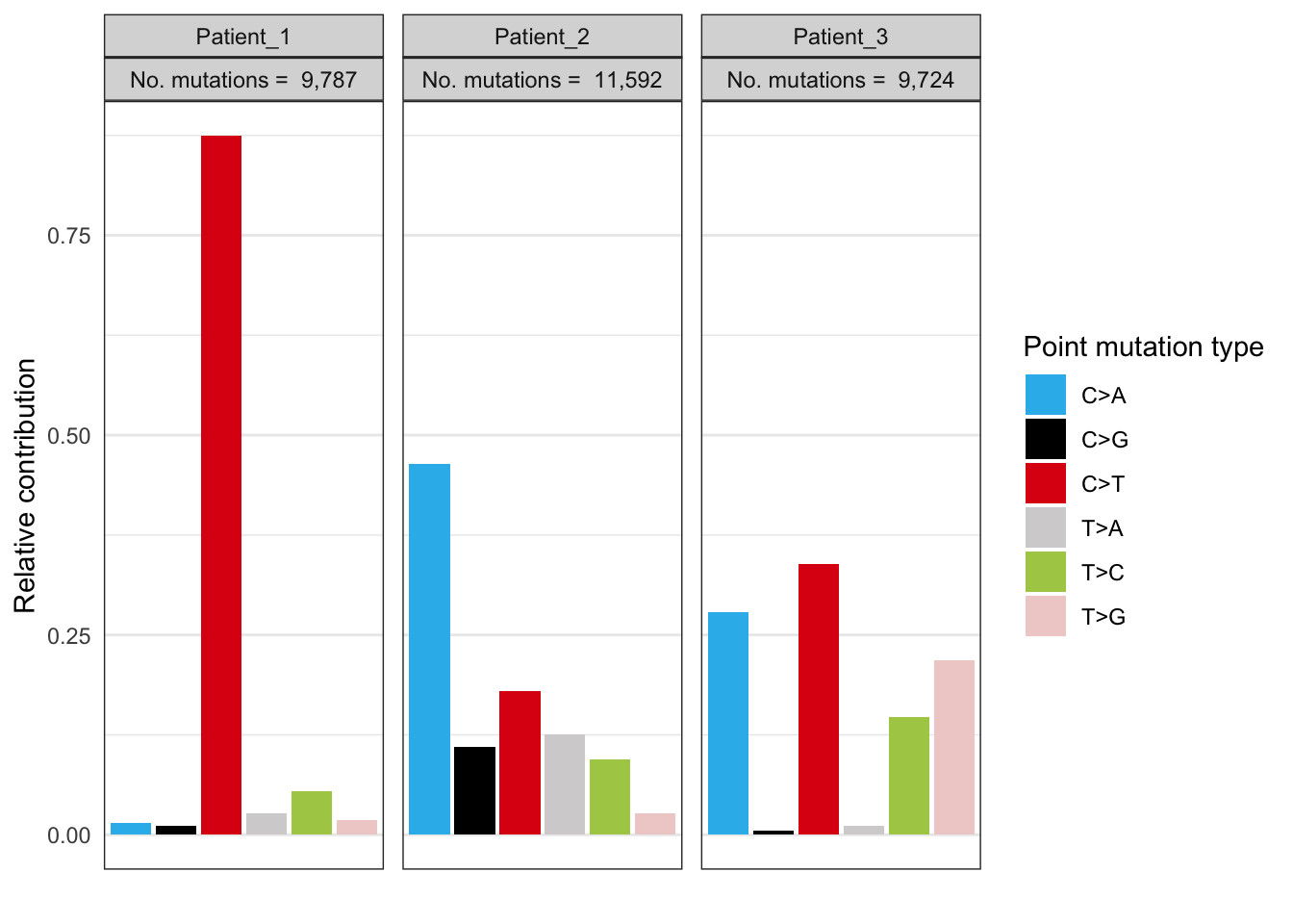
Explore mutation contexts
For mutational signature analysis, we have to characterize the
trinucleotide context of each point mutation to construct the 96
trinucleotide mutation count matrix. The mut_matrix
function does this for you.
EX1_mut_mat <- mut_matrix(vcf_list = EX1_vcfs, ref_genome = ref_genome)
head(EX1_mut_mat)
## Patient_1 Patient_2 Patient_3
## A[C>A]A 12 450 12
## A[C>A]C 12 281 23
## A[C>A]G 1 126 1
## A[C>A]T 11 329 48
## C[C>A]A 21 649 36
## C[C>A]C 5 608 16Next, you can use this matrix to plot the 96 profile of samples.
EX1_plot_profile <- plot_96_profile(EX1_mut_mat) ## Warning in geom_bar(stat = "identity", colour = "black", size = 0.2): Ignoring unknown parameters: `size`EX1_plot_profile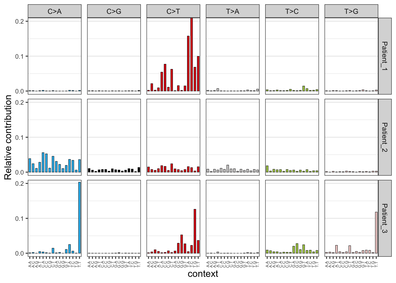
These 96 mutational profiles represent all the mutations of every mutational process that has been operative in the cancers of the 3 cancer patients. The 3 patients show a completely different 96 mutation profile which indicates that different mutational processes have been operative in these 3 tumors. For instance, the third patient has accumulated 20% (look at y-axis) C>A mutations but only when a T is located left and right of the mutated cytosine T[C>A]T. The second patient also received many C>A mutations but with a less strong trinucleotide bias. The first patient only acquired C>T mutations.
Extract the mutational signatures
To identify which mutational processes have been operative in these 3
samples, we can fit the 96 mutational profiles to the known COSMIC
signatures. Signature refitting quantifies the contribution of the
signatures to the mutational profile. For this, we can make use of the
fit_to_signatures function. This function fits the mutation
matrix to cancer signatures. First, we need to load the COSMIC
signatures:
signatures = get_known_signatures()
#double check whether this is a 96 matrix. The columns represent the number of signatures.
dim(signatures)
## [1] 96 60And run the fit analysis:
EX1_fit_res <- fit_to_signatures(EX1_mut_mat, signatures)Take a look at the results:
head(EX1_fit_res$contribution)## Patient_1 Patient_2 Patient_3
## SBS1 57.54215 25.86982 0
## SBS2 0.00000 130.44682 0
## SBS3 0.00000 0.00000 0
## SBS4 0.00000 6459.36306 0
## SBS5 0.00000 0.00000 0
## SBS6 0.00000 0.00000 0This matrix contains the absolute mutational contribution of
each mutational signature (row) per patient (column). For instance,
57.54215 mutations are assigned to SBS1 in patient 1, whereas 25.86982
mutations are assigned to SBS1 in patient 2. However, the absolute
number of mutations must always be an integer number. It is important to
realize that this function computes the best linear fit of a
mathematical approach and these non-integer numbers must be interpreted
as computational estimates. In mutational signature analysis we
typically apply the round() function to the computational
estimates to better represent the absolute mutational contributions of
mutational signatures.
head(round(EX1_fit_res$contribution))## Patient_1 Patient_2 Patient_3
## SBS1 58 26 0
## SBS2 0 130 0
## SBS3 0 0 0
## SBS4 0 6459 0
## SBS5 0 0 0
## SBS6 0 0 0We observe that 58 mutations are attributed to SBS1 in patient 1, and
26 mutations in patient 2. Apparently, more than 6000 mutations are
linked to SBS4 (smoking signature) in patient 2. To reveal which
mutational signature represents most of the mutations in each sample, we
need to calculate the relative contributions. The
plot_contribution function can do this with
mode = "relative".
# plot contribution
EX1_plot_refit <- plot_contribution(EX1_fit_res$contribution,
                    signatures,
                    coord_flip = FALSE,
                    mode = "relative" )
EX1_plot_refit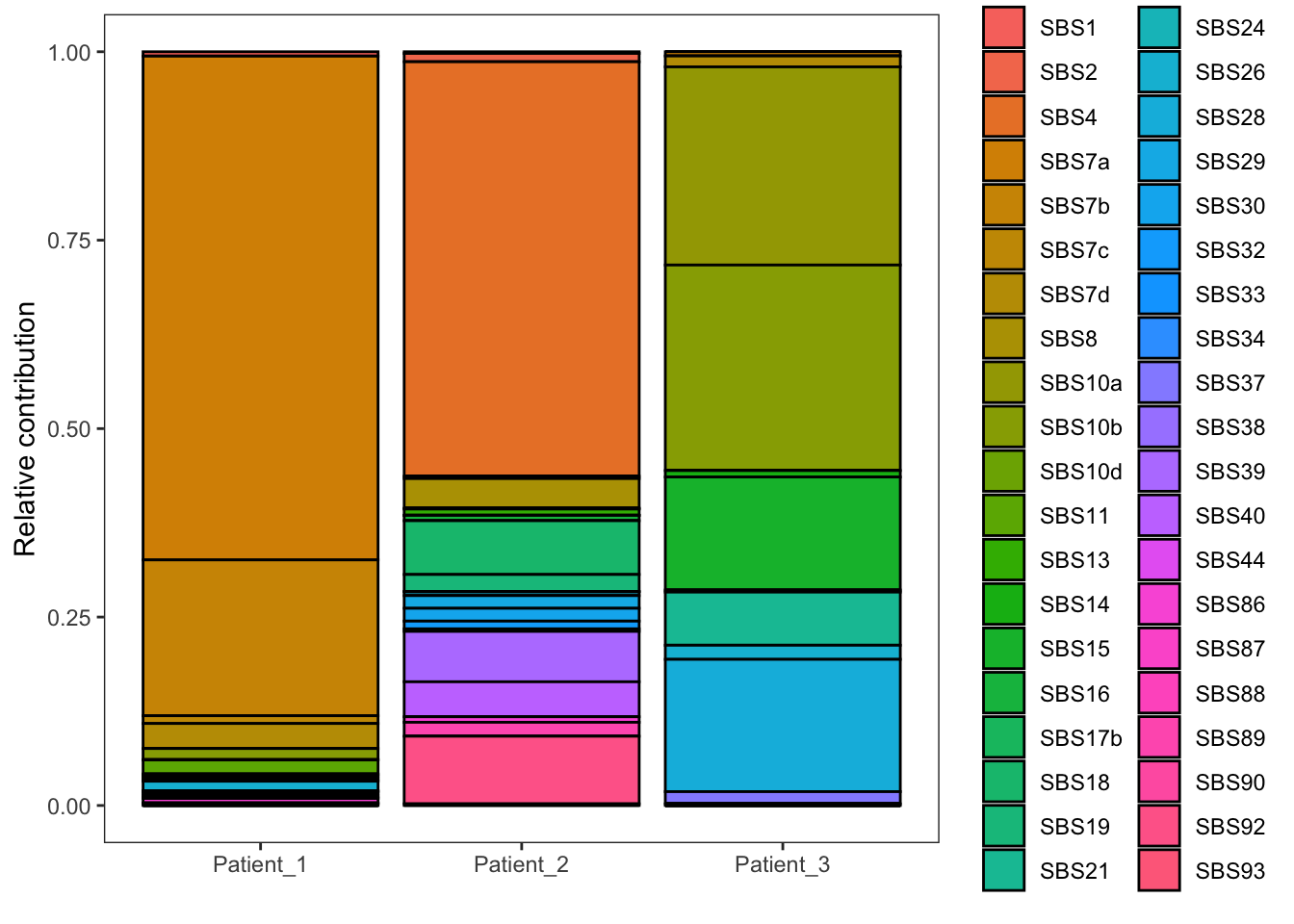
The y-axis represents the relative contribution of each signature. A relative contribution of 25% means that 25% of the mutations can be attributed to that mutational signature (ie the mutational process of that signature has induced 25% of the total number of mutations in that cancer sample). As you can see, we observe contributions of many signatures with some signatures showing a high contribution (e.g. > 10%), while others show a more limited contribution. We know that only a moderate number of mutational processes typically operate in cancers, thus the signatures with low contributions are artefacts. The explanation behind these artefacts is that we are looking at a fit that statistically gives the best result, and this purely mathematical approach does not take into account biological interpretation. This problem, known as overfitting, occurs because fit_to_signatures finds the optimal combination of signatures to reconstruct a profile. It will use a signature, even if it improves the fit very little.
One way to deal with overfitting is by starting with a standard refit
and then removing signatures that have little contribution on how well a
mutational profile can be explained. This works in an iterative fashion.
In each iteration the signature with the lowest contribution is removed
and refitting is repeated. In MutationalPatterns it can be
assessed with the fit_to_signatures_strict function.
# plot contribution
EX1_strict_refit <- fit_to_signatures_strict(EX1_mut_mat, signatures, max_delta = 0.004)
EX1_fit_res_strict <- EX1_strict_refit$fit_res
EX1_plot_strictrefit <- plot_contribution(EX1_fit_res_strict$contribution,
                  coord_flip = FALSE,
                  mode = "relative"
)
EX1_plot_strictrefit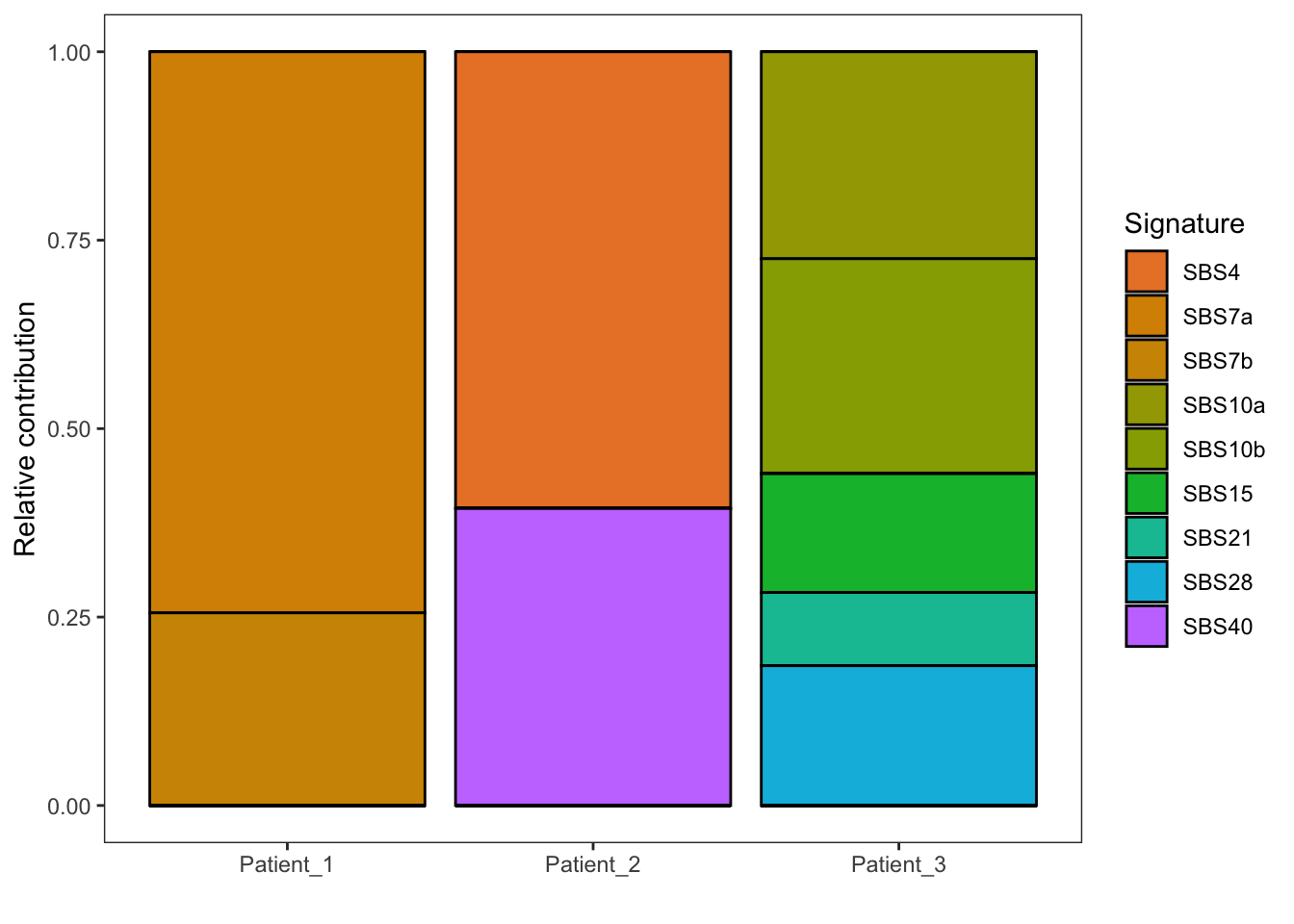
Compared to the previous plot, only the most dominant (true) mutational signatures are displayed. Thus, from all the point mutations in the raw data file (VCF) we are able to retrieve the activity of the most dominant mutational processes. Please fill in the questions below. You will need the link to COSMIC SBS signatures and COSMIC DBS signatures to look up the etiology of each signature.
Exercise 1c: What is the dominant mutational signature of patient 1?
Exercise 1d: What is the mutational proces of this mutational signature in patient 1?
Exercise 1e: What is (probably) the primary tumor type of patient 1?
Exercise 1f: What is the dominant mutational signature of patient 2?
Exercise 1g: What is the mutational proces of this mutational signature in patient 2?
Exercise 1h: What is (probably) the primary tumor type of patient 2?
Exercise 1i: What is the dominant mutational signature of patient 3?
Exercise 1j: What is the mutational proces of this mutational signature in patient 3?
Exercise 1k: What is (probably) the primary tumor type of patient 3?
Exercise 2
In Exercise 2, you will need to read in and work on the VCF file of one patient and explore the SBS and DBS mutational signatures. Here, you will rely on the code from Exercise 1 that needs to be adjusted to answer questions from Exercise 2.
Import file for exercise 2.
# Import mutation data from VCF files
# Don't forget to change the path to the files
EX2_vcf_files <- list.files(
  path = getwd(),
  pattern = "EX2",
  full.names=TRUE)
Exercise 2a: What is the dominant SBS mutational signature of this patient?
Exercise 2b: What can you conclude from the mutational signature
analysis of this cancer sample?
Instead of point mutations, we can also assess the double base substitutions (DBS - a mutation type where 2 flanking nucleotides are mutated). Can you perform a DBS mutational signature analysis on this sample? Use the manual to find the code you need to perform DBS mutational signature analysis.
TIPS:
- When you load the mutations with the
read_vcfs_as_grangesfunction, you have to addtype = "dbs"and thepredefined_dbs_mbs = TRUE.
- You have to obtain the DBS_context using
get_dbs_context()andcount_dbs_contexts.
- The DBS signatures can be loaded with
get_known_signatures(muttype = "dbs").