COO R
T Huisman
2025
Introduction
This is a small refresher on basic R skills, based on the exercises from the prior course Onderzoeksmethoden. For quick help with syntax and functions, refer to the basic R cheatsheet or built-in documentation via the help function (add a question mark in front of the function).
We will be doing a short data analysis to cover all the important
skills you’ll need. Make sure you work in the code editor panel
and save your script often. Add commentary lines (starting with
#) for additional context. Your final script should be
sufficient to perform and understand the analysis described on this
page.
Learning goals
- (General)
- The student can write a basic R script and edit code in Rstudio
- The student can create and store plots, data and scripts
- Variables and Data Structures
- The student can make, name, and use data objects in R
- Functions
- The student can apply functions and enter the correct arguments
- Loading Data
- The student can load a variety of common data formats
- Subset
- The student can make a selection or subset of data
- Plot
- The student can make and configure basic plots
- %in% Operator
- The student understands the %in% operator
- Iteration
- The student can apply looping functions
apply(),lapply(),sapply(), and so on - The student can apply and explain simple for-loops
- The student can apply looping functions
1. Load data
The research question for these exercises:
Are Notch signaling pathway genes differentially expressed between virgin and lactating mice?
We will use the RNA expression profiles of basal stem-cell enriched cells (B) and committed luminal cells (L) in the mammary gland of virgin, pregnant and lactating mice. The data is adapted from Fu NY, Rios AC, Pal B, Soetanto R et al. 2015 \(^1\). This is RNA-seq data, which will be explained in a later part of the course (COO-RNAseq). For now, all you need to know is that the number data represent expression level per gene (rows) in different samples (columns). Six groups are present, with one for each combination of cell type and mouse status. Each group contains two biological replicates.
You will need the following files, save them into a folder of your choice: Use Right-mouse click > ‘save link as …’
Next, set your working directory to the folder that contains these data files. Click on the RStudio toolbar ‘Session’ >> ‘Set working directory’ >> ‘Choose directory’ or hit Ctrl+Shift+H on your keyboard. Take note of the line of code that appears in the R Console afterwards. You need to put this line in your R script. It looks like the code below, except with the path to your data folder. See OZM COO2 for a quick refresher.
setwd("~/Documents/Bioinformatica/COO-R")Load the Sample information from the
SampleInfo_Corrected.txt file using the code
below.
sample_info <- read.delim("SampleInfo_Corrected.txt")
sample_info
SampleName CellType Status
1 MCL1.DG basal virgin
2 MCL1.DH basal virgin
3 MCL1.DI basal pregnant
4 MCL1.DJ basal pregnant
5 MCL1.DK basal lactate
6 MCL1.DL basal lactate
7 MCL1.LA luminal virgin
8 MCL1.LB luminal virgin
9 MCL1.LC luminal pregnant
10 MCL1.LD luminal pregnant
11 MCL1.LE luminal lactate
12 MCL1.LF luminal lactateQ1a) What field separator character is used by
read.delim for reading in our sample_info? Is
there a header line for column names in
SampleInfo_Corrected.txt?
Check if the data is loaded correctly. Make sure your
sample_info properly matches ours. There are a bunch of
functions to quickly check the important properties of your data
object.
head(sample_info)
class(sample_info)
str(sample_info)
dim(sample_info)
Q1b) What sort of data structure is the
sample_info object? What are the basic types of each
column?
We should also load the actual expression data from the
GSE60450_Lactation-GenewiseCounts.txt file.
countdata <- read.delim("GSE60450_Lactation-GenewiseCounts.txt")Q1c) What do the first two columns of countdata
describe?
Q1d) How many genes (rows) and samples (columns) are recorded in the count data?
2. Bad Columns
Q2a) Make a new named object onlycounts that
contains all but the first two columns of
countdata.
# Please complete the code below to only select the sample columns of countdata
onlycounts <- countdata[ , ]
Q2b) Check the remaining columnnames, it should match our columnnames below.
colnames(onlycounts) [1] "MCL1.DG" "MCL1.DH" "MCL1.DI" "MCL1.DJ" "MCL1.DK" "MCL1.DL" "MCL1.LA" "MCL1.LB" "MCL1.LC" "MCL1.LD" "MCL1.LE" "MCL1.LF"3. Fix Row Names
The rownames of onlycounts should match the
EntrezGeneID column of the original countdata
object. We use these names to select data later on.
Q3) Replace the rownames of onlycounts with the
gene IDs from the original countdata.
# Please complete the code below to replace the rownames with the gene IDs from countdata
rownames(onlycounts)
4. RPM
Raw countdata is not suited for plotting or statistical analyses. Some samples were sequenced deeper than others, resulting in more reads per gene and a greater so-called library size. We should normalize the countdata to correct for such technical differences. To this end, we will perform a couple of steps to calculate the Reads Per Million (RPM), which are better suited for plotting and analysis.
# Tiny toy example, say we have sample 1 and 2 with these readcounts
(reads <- rbind(c(20,10), c(35, 20), c(15,15)))
[,1] [,2]
[1,] 20 10
[2,] 35 20
[3,] 15 15# You'd think sample 1 has more reads for each gene (row) and higher expression than 2
# But note the readcount total (library size) per sample. This is a technical difference.
# Total reads: 70 and 45 respectively.
# Dividing the reads by their respective sample total is more insightful! [,1] [,2]
[1,] 0.2857143 0.2222222
[2,] 0.5000000 0.4444444
[3,] 0.2142857 0.3333333In programming we often have to perform the same function or
operation many times over: it’s called iteration. There is a family of
apply() functions to perform functions on each row or
column.
Q4a) Calculate the total sum of readcounts in
onlycounts per sample and call the vector
SizeFactor. Explain each part of the example code
below.
SizeFactor <- apply(onlycounts, 2, sum)Q4b) Divide the SizeFactor by a million. This is the “Per Million” part of RPM.
SizeFactorM <- SizeFactor / 1e6Q4c) Next, we divide the columns of countdata by their
respective size factor. Note that there are several ways to do this.
This is just one code example using the sweep function that
is quite similar to apply. The division operator "/" is
applied to the columns. You don’t need to know this sweep
function.
RPM <- sweep(onlycounts, 2, SizeFactorM, "/")5. Filter Genes
It is customary to exclude genes when the combined total RPM of the gene in all the samples is low. This selection is based on the sum of rows.
Q5a) Use the apply function to calculate the
total RPM per gene. What MARGIN and FUN
arguments should you use?
# Please complete the code below to calculate row sums
totalRPM <- apply(RPM, , )
Q5b) Check if the total RPM of each gene is lower than 5.
totalRPM < 5Q5c) How many genes have a total RPM lower than 5?
Hint: Use the table() function to count the number of
TRUE and FALSE in your output.
table(totalRPM < 5)Q5d) Make a subset of RPM that contains only
genes with a total RPM of at least 5. Store this subset in
filteredRPM. How many rows should be in the final
filteredRPM?
# Complete the code below
selected_genes <- totalRPM >= 5
filteredRPM <- RPM[ , ]
6. Plot Data
Q6a) Make a box plot of the filteredRPM with a
box per sample.

This plot is not very clear. We will log-transform the RPM data to
make nicer plots and to perform downstream analyses. We add a
pseudo-count +1, because log(0) gives an
error.
Q6b) Calculate the logRPM.
logRPM <- log(filteredRPM + 1)Q7c) Make a box plot of the logRPM with a box
per sample. Color the boxes per cell type. Hint: We use the
information from sample_info. The factor essentially gives
each group a number, and these numbers correspond to colors in R.
boxplot(logRPM, main = "log RPM", col = as.factor(sample_info$CellType))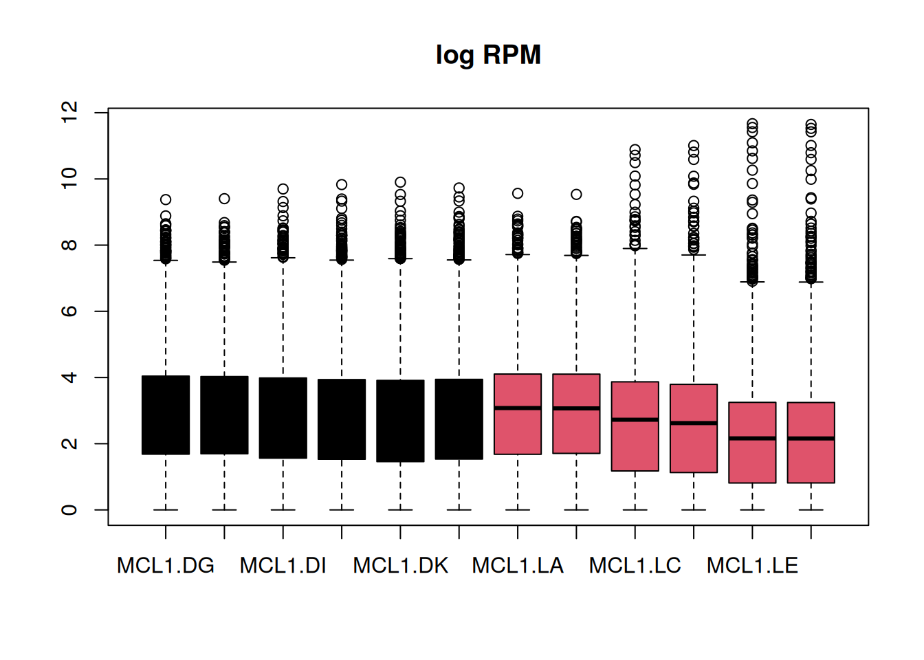
Q7d) Make a box plot of the logRPM with a box
per sample. Color the boxes per mouse status.
# Please complete the code below to color the boxes by mouse status
boxplot(logRPM, main = "log RPM", col = )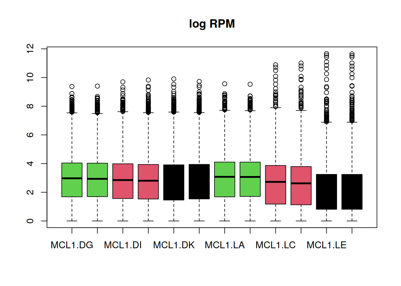
7. Investigate Pathways
Q7a) Look for the “Notch1” gene of house mouse (Mus musculus) on https://www.ncbi.nlm.nih.gov/. You should find a hit with Entrez ID “18128”.
Q7b) Is EntrezGeneID “18128” present in logRPM?
Explain the code below.
"18128" %in% rownames(logRPM)[1] TRUEQ7c) Go to the “Signaling by NOTCH” page listed in the “Pathways from PubChem” section of the Notch Gene NCBI page. Find the Genes section of the Signaling by Notch PubChem page. Download the data table and save it in your working directory. If you are having trouble, you can use this file we prepared earlier: pubchem_pathwayid_14079_pcget_pathway_gene.csv Don’t “open with Excel”. First download the files to your system. Excel changes the contents of files!
Q7d) Load the Notch genes table into R. How many genes does it have and what do these genes represent?
Signaling by Notch genes
We start looking into the Signaling by Notch genes data.
Q7e) Store the gene Ids column from the gene table as a
separate vector genes.
Q7f) Check if each gene of genes is present in
logRPM.
Q7g) Before we continue, make a subset of the
logRPM and sample_info that only contains info
on the "virgin" or "lactating" mice by
excluding the "pregnant" mice data.
subdata <- logRPM[, sample_info$Status != "pregnant"]
subinfo <- sample_info[sample_info$Status != "pregnant",]
Q7h) Make a box plot of the logRPM values of
Notch1, entrez ID “18128”, with a box per mouse status. See also OZM
COO3 for a refresher on plotting syntax.
plot(as.numeric(subdata[rownames(subdata) == "18128",]) ~ as.factor(subinfo$Status), main = "Notch1", xlab = "Mouse Status", ylab = "log RPM")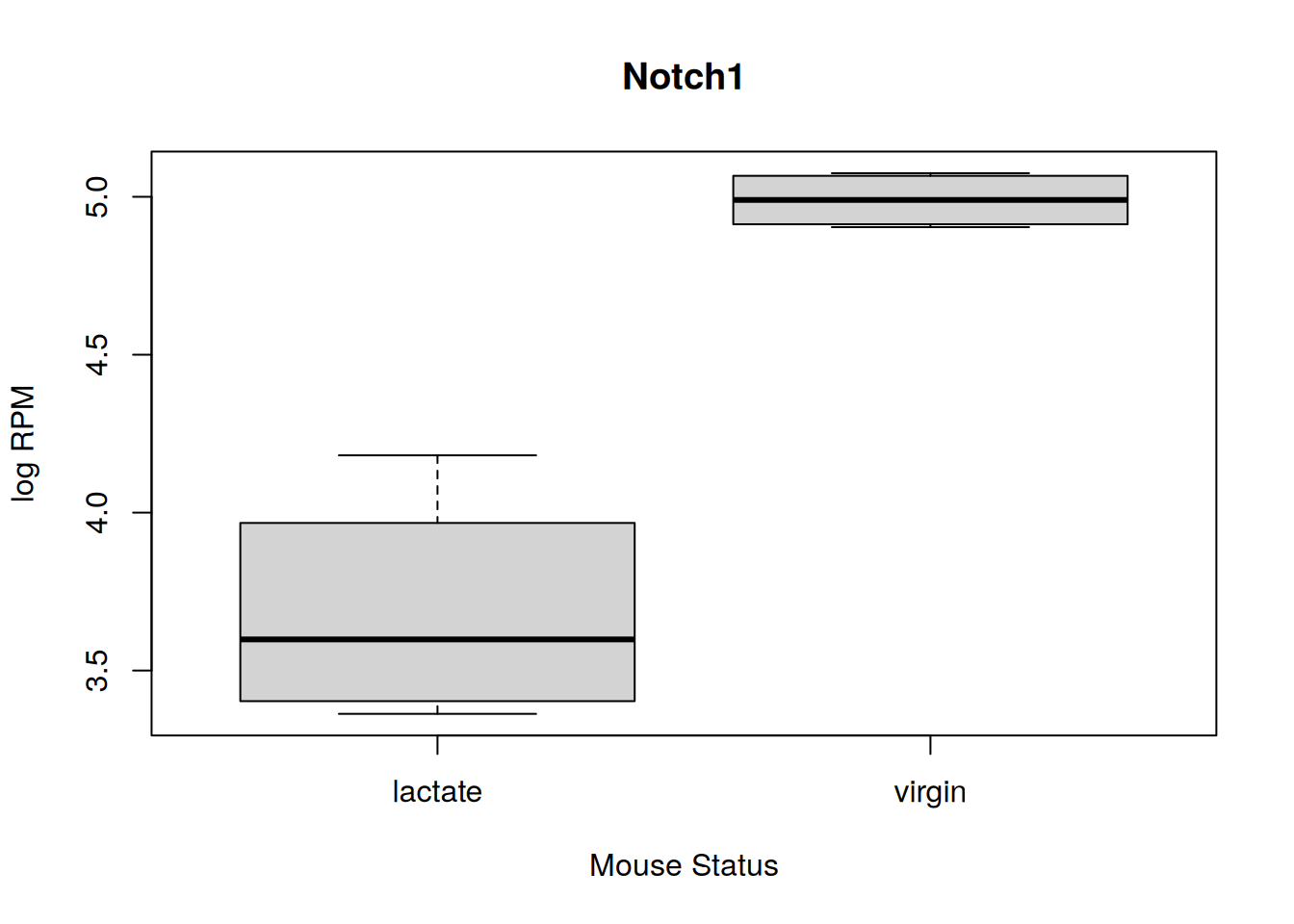
The for-loop is a construct used for iteration. The code inside the for-loop is repeated once for every element of a sequence specified in the for statement. The iterating variable takes on the value of the current element each loop.
Q7i) Plot the log RPM of the first five genes in
subdata. Explain the example below.
(This code generates multiple box plots - one for each of the first five genes. Use the left/right arrow icons of the Plot panel to switch between the generated boxplots.)
for (row in 1:5) {
  boxplot(as.numeric(subdata[row,]), main = rownames(subdata)[row], ylab = "log RPM")
}
Q7j) Make a box plot of the log RPM subdata for
each Signaling by Notch gene in genes. Make a box per Mouse
Status. Explain the code below.
(This code generates multiple box plots - one for each gene in the Notch signalling pathway. Use the left/right arrow icons of the Plot panel to switch between the generated boxplots.)
for (gene in genes) {
  boxplot(as.numeric(subdata[rownames(subdata) == gene,])  ~ as.factor(subinfo$Status), main = gene, xlab = "Mouse Status", ylab = "log RPM")
}
Q7k) Use the following statistical test to determine if the difference in gene expression of gene “66354” is statistically significant.
v <- subdata["66354", subinfo$Status == "virgin"]
l <- subdata["66354", subinfo$Status == "lactate"]

t.test(v,l)
    Welch Two Sample t-test

data:  v and l
t = 3.4233, df = 4.3375, p-value = 0.0235
alternative hypothesis: true difference in means is not equal to 0
95 percent confidence interval:
 0.1138589 0.9540301
sample estimates:
mean of x mean of y
 4.229219  3.695275
Q7l) Look at the “Signaling by Notch” gene boxplots, which one of these genes appears upregulated in lactating mice compared to virgin mice? See if you can find out if this gene and its expression is linked to lactogenesis in literature.
8. Final Remarks
Save the script. Make sure your script is complete and you’ve added comments where necessary. Close the RStudio window. Don’t save the workspace image. Afterwards open your script and run all (hit Ctrl+Shift+Enter on your keyboard). Does everything work without throwing errors? If not, adapt your code and try each step of the analysis again until your whole script runs without error. This is the ultimate proof of reproducibility, nice for yourself, future coworkers, and science.
Install the required R packages
Download install_bioinf.R and open this script in RStudio. Follow the instructions inside the script.
\(^1\) Fu NY, Rios AC, Pal B, Soetanto R et al. EGF-mediated induction of Mcl-1 at the switch to lactation is essential for alveolar cell survival. Nat Cell Biol 2015 Apr;17(4):365-75.