COO1 - Introduction R

During the course, we will work often in RStudio. In this computer module, you will install RStudio and learn about the basics of R.

1. Install and work in RStudio

You can download R and RStudio by following the steps below.

Go to https://cran.r-project.org/ to download R
Select your operating system (OS)

Windows: choose ‘base’, and download and install R
MacOS: download the most recent package
Linux: choose your distribution and follow the instructions

After installing R, you can install RStudio
Go to rstudio.com
Download and install the free version (open source edition) of RStudio Desktop for your OS

When starting RStudio for the first time, it might ask where you installed R (in step 2)

Note that R also comes with an application called RGui, but we will not use this during the course. We will only use RStudio.

Throughout this and future COOs, we assume you work on Windows. We will demonstrate the use of keyboard shortcuts, like pressing Ctrl+Enter to execute a script. If you use Mac, keyboard shortcuts can be different. In this specific case, you should use Cmd+Return. A list of all keyboard shortcuts for all operating systems can be found in RStudio under Tools → Keyboard Shortcuts Help.

RStudio contains 4 panels:

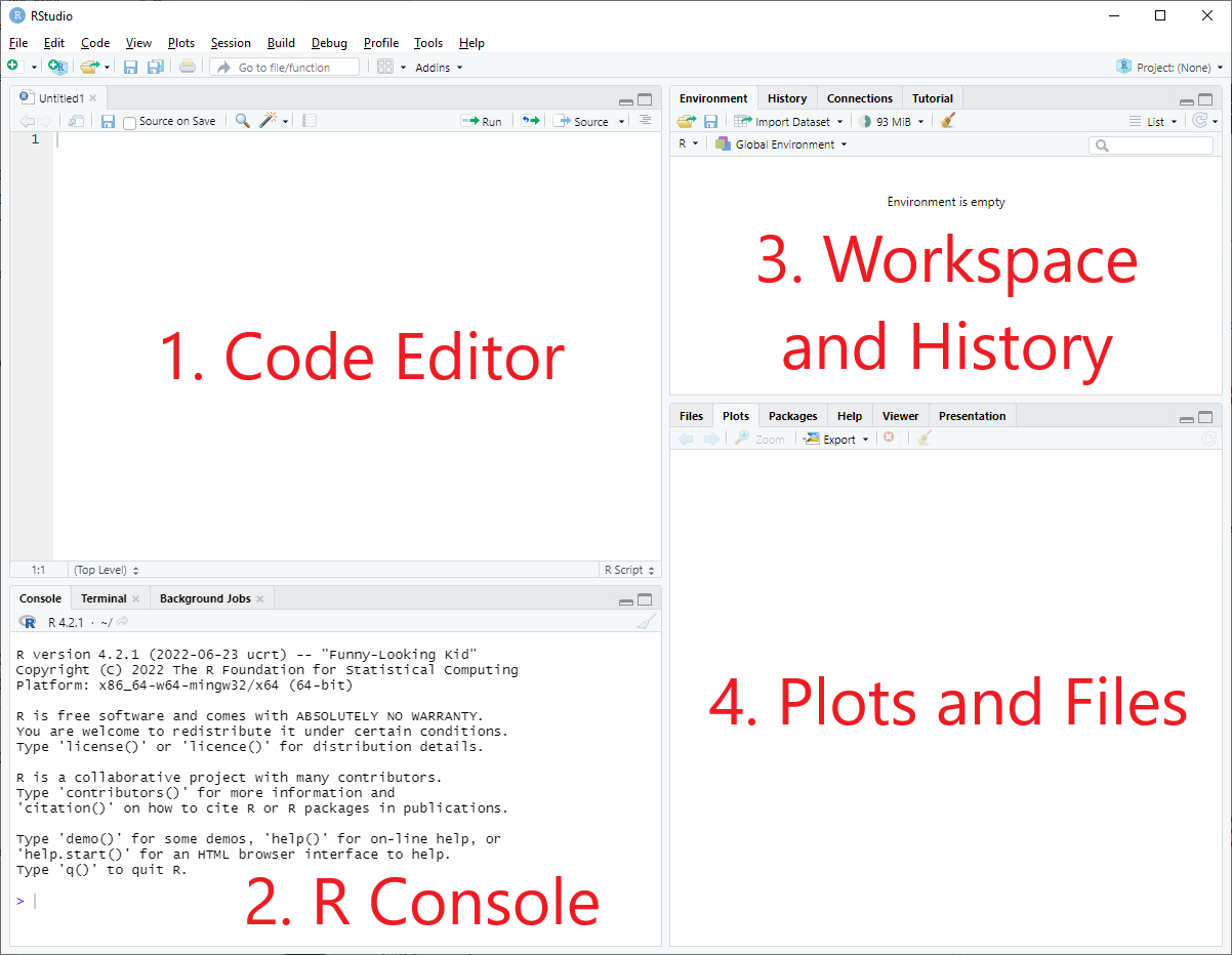
The Code Editor in which you write your script. This panel will only appear when you have created a new file by clicking File → New File → R Script. The script is your ‘work document’ which can be saved for later use, so it’s important to always write your code in a script and not directly in the R console (see 2).
The R Console in which your script is executed and where the results are shown. You can also write and execute code here instead of in the script, but this is not recommended (see 1).
The interactive Workspace and History contain the objects you will create during this tutorial.
In the Plots and Files panel, you can find ‘files’, ‘plots’, ‘list of packages’, ‘help’, ‘viewer’, and ‘presentation’.

To find help, you can click ‘help’ and search for a certain topic. Alternatively, you can type and execute a questionmark and the name of the function in your script, e.g.: ?read.table. In the ‘help’ section you can search specific questions, which will direct you to an information page. If this does not satisfy what you were looking for, it is encouraged to search the internet, ask ChatGPT, a fellow student, or a teaching assistant (in that order).

This manual shows step by step what is expected of you to write in your script. You can copy-paste it, but it is better to write it yourself. You will see why this is so important in following tutorials in which we will write more complex scripts. Slight mistakes, for instance typo’s or uppercase vs. lowercase letters, alter how your script works and it may not give the desired output. When you have written a script, you can press run or press Ctrl+Enter to execute the code.

R code is executed in the Console, meaning that the output will be displayed in the Console. The blue greater-than-sign (\(\color{blue}{>}\)) on the very last line of the console is a so-called command prompt and it indicates that R is ready to receive commands (i.e., through the code you write and execute in your script). If you enter an incomplete line of code, you instead get a blue plus sign (\(\color{blue}{+}\)) prompt on the next line in the Console. This means R is expecting you to enter additional information to finish the incomplete code before you can continue. You can stop this by clicking in the Console panel in the line with the plus sign (\(\color{blue}{+}\)) and pressing Esc.

2. R calculations and assignments

Below starts a tutorial that teaches you all the basics you need to know to understand how RStudio works. From now on, everything in the grey area is what is expected of you to write in your own script opened in the Code Editor. The white line underneath starting with [1] will give you the expected answer as displayed in the Console. If you failed to provide the same answer, try to find what went wrong, Google your problem, or ask ChatGPT or any of us for help. Exercises are displayed in bold.

2.1 Simple calculations

We will start by practicing some more simple calculations below. Type and execute the following in your R script (the upper left panel). The output will be displayed in the Console (the lower left panel):

8 - 4

[1] 4

9 / 3

[1] 3

9 : 3

[1] 9 8 7 6 5 4 3

The -, /, and : symbols are examples of operators. The operator : does not give the same outcome as the / operator. The - and / are examples of so-called Arithmetic Operators; while the : is a so-called Colon Operator. In RStudio the Arithmetic Operators (like / and +) perform mathematical operations such as addition, subtraction, multiplication, division, etc. The Colon Operator (:) returns a sequence of numbers within a closed interval specified by the numbers before and after the operator, in this example all numbers between and including 9 and 3.

A multiplication in RStudio is an * operator.

4 * 4

[1] 16

1. Now multiply 5 times 8

Some other calculations:

7 ^ 2

[1] 49

(10 + 5)  * 3 #everything within the parentheses will be executed first

[1] 45

In R you can add notes by using the #, which could for instance be useful to explain what you wrote down in the script and why, how the code works, to comment on parts where you did something wrong or to mark the beginning of a new part. Everything behind the # will be ignored by R. It is very important to structure your script like this, because it helps you understand your scripts in the future and helps others to use and adapt your scripts as well. #this is just a note and R will ignore it

2.2 Assigning a value to an object name

2. What happens if you type the following in the code editor (upper left panel):

1 + 2 and press Enter.

3. What happens if you type:

1 + 2 and then press Ctrl+Enter

The outcome of your calculation will only appear in the R console if you run it. Now that we have covered some simple calculations, we can assign values to object names. An object is a data type in which a value or any information can be stored digitally. This can be done using a left arrow operator: <- (a less-than character < followed by a minus character -). All objects you create and store will appear in the Workspace and History panel (upper right), under the Environment tab. There are three ways to create an object, which you can try out below. From now on no answers will be shown so you have to write them down and correct them later on, if needed.

a <- 3 #If you run this 'a <- 3' will appear in the R Console (lower left panel). The object 'a' now stores the value '3'. If you then type 'a' in your script and run it, the value '3' will appear. The object 'a' will be shown in the Environment tab (upper right panel).
a

The object ‘a’ with value ‘3’ is now stored.

Note that you can also use an equal sign (=) or a right arrow (->), which you might encounter in code written by others and looks like this:

a = 3
a

3 -> a #the arrow always points to the object name to store the value or other information properly
a

It is very important to be consistent in the operator you use; choose one. For this course we will always use <-.

We can also do simple calculations with our newly formed objects:

a - 2

a * 16

a <- 8
a

Note that it is possible to overwrite your objects. By running the a <- 8 command, you can now see in your upper right panel (Environment tab) that your value for a has changed from 3 to 8. It is thus better to store different values under different object names, so you can use both 3 and 8 with a unique object name (for example a and b).

b <- 6 + 12
b

4. What do you think will be the answer to the following?

a + b

3 Different data types

There are different types of data, the most basic types are depicted in the table below.

Data type	Literal
Logical	`TRUE` or `FALSE`
Numeric	`1`, `2`, `3.5`, `-6`, `1.2e3`
Character	`"Name"`, `'Word'`

To see what kind of data type an object in R is, you can use the command class(). So, for example, if you run class(TRUE), it will return [1] "logical".

3.1 Logical data

Logical data only has one of two possible values, often depicted as TRUE or FALSE (or 1 and 0). The logical data type tells you whether something is true or not. For example: you can ask R whether one value is greater than another value. When this is true, R will return ‘TRUE’. To make different comparisons, you can use the following relational and logical operators:

Operator	Description
`<`	Less than
`>`	Greater than
`<=`	Less than or equal to
`>=`	Greater than or equal to
`==`	Equal to
`!=`	Not equal to
`&`, `&&`	And
`\|`, `\|\|`	Or

The comparison operators (top six rows) are called the Relational Operators. The operators ‘and’ and ‘or’ belong to the Logical Operators.

The logical operators come in a shorter form (&, |) and a longer form (&&, ||). If you are performing logical comparisons on lists of data (e.g. a vector; this will be explained later in this course), there are important differences between them that can be found in the documentation. When in doubt, use the longer form. There are two additional logical operators: ! is logical negation (!FALSE == TRUE) and xor(x, y) for the exclusive or (only x or y is true, but not both).

Try the following statements:

1 > 2 #This means that you want to check whether 1 is greater than (>) 2, which is not the case and returns FALSE.

2 > 1 #This means that you want to check whether 2 is greater than (>) 1, which is correct and returns TRUE.

1 < 2 #This means that you want to check whether 1 is smaller than (<) 2, which is correct.

1 <= 2 #This means that you want to check whether 1 is smaller than or equal to 2, which is correct.

2 <= 2 #This returns TRUE because '2' is equal to '2'.

2 >= 3 #This means that you want to check whether 2 is greater than or equal to 3, which is incorrect because 2 is smaller than 3.

We can then ask R the same questions as before but now using a predefined object ‘x’.

x <- 5
x > 4

Because ‘x’ now stands for ‘5’ the question is whether ‘5’ is greater than ‘4’ which is correct, and R therefore returns TRUE.

To check whether x is exactly 5, you can use:

x == 5

Note that while x = 5 is a command to assign the value ‘5’ to the object ‘x’, x == 5 is a command to compare the two objects.

5. What do you expect to return when you use the following command?

x == 4

We can also do the opposite and ask R if ‘x’ is not equal to ‘4’ with !=.

x != 4

x != 5

It is very important to place spaces between the object name and operators since x<-5 can mean that you want to assign ‘5’ to ‘x’ (e.g., x <- 5) but if you do not space it properly (e.g., x< -5), it says that ‘x’ is smaller than ‘-5’:

x < -5

3.2 Numeric data

Examples of numeric data include actual numbers such as 1, 2, 3 and 3.5. If you execute class(3.5) R will return [1] "numeric". The class function can tell you the datatype of your object. Note that decimals must be indicated with a period and not with a comma, as R uses a period as decimal seperator and a comma for listing. For example, if you command R to return class(3,5), you ask to return the class of both ‘3’ and ‘5’. This will return an error, as it can only assess the class of one object at a time. A subclass of numeric data is the data type ‘integer’. Integers are “whole” numbers, for example 1, 163, and -15. Fractions, such as 1/2, 9.13, and the square root of 2, are of the data type numeric, but not of the data type integer.

You may encounter somewhat more exotic number formatting in real life code. For completeness, we are showing them here as well. First the scientific notation, in which for instance 1200 is written as 1.2×10³. In R this is written as:

1.2e3

[1] 1200

3.3 Character data

The data type ‘character’ is used for text or so-called string values. An example of character data would be your name or a string object X. Character data is presented between quotes, for example “Thomas”. class("Thomas") and class('Thomas') will return [1]"character". If you forget the quotation marks, R interprets Thomas as an object. Since you didn’t create an object called Thomas, R will return an error message for class(Thomas). The color of the text in your script changes according to its class. This will make you notice when you start a character string (with "), but forget to close it with another quotation mark.

Note that you have to use the plain quotations marks ' or ". The nice quotation marks (‘ ’ or “ ”) that Word or other editors use will cause an error in R.

4 Vectors

A vector is a sequence of the same data type. To make a vector, you can use logical, numeric or character data. The vector starts with c() followed by the data sequence. The c() function is used to combine different elements. You separate the elements in a vector with commas.

c(1, 2, 3, 4)

Now you created a vector but when you want to continue to use this vector, R cannot recall them. Therefore, we must assign the vector to an object name.

vector1 <- c(1, 2, 3, 4)
vector1

Now you can use the object vector1 to use the numeric data from your vector.

vector2 <- c(2, 3, 4, 5)
vector2

You can do some simple calculations with two different vectors:

vector1 + vector2

c(1, 2, 3, 4) + c(2, 3, 4, 5)

You will notice that the first element of the first vector will be added to the first element of the second vector (1+2), the second to the second (2+3), and so on, to return a new vector (3,5,7,9). You can also apply one type of calculation to every element in the vector:

vector1 + 3 #adding three to every element in vector1.

vector2 * 2 #multiplying every element in vector2 by two.

6. Write a line of code to subtract 4 from each element of vector1.

7. Write code to divide each element of vector2 by 5.

4.1 Vectors using a colon

You can also make vectors with the sequences of integers (“whole” numbers) using the Colon Operator (:):

vector3 <- 1:10
vector3

The colon operator can be used to display all datapoints between 1 and 10. We do not need to use the c() function to make such a numeric vector.

vector4 <- 10:1
vector4

8. Try making a very large vector (e.g. ranging from 13 to 524) and a vector of negative values (e.g. ranging from -20 to -50; or -10 to 8).

4.2 Vectors using functions seq() and rep()

Vectors can also be created using seq() (sequence) or rep() (repeat) functions. We have already used some simple functions before, for example the c() command to create vectors. Each function contains one or multiple arguments. These arguments are stated between the brackets of the function. The sequence generation function seq() creates a regular sequence:

seq1 <- seq(from = 1, to = 5, by = 0.5) 
seq1

As you can see, seq1 is a vector which starts with 1 and then follows up to 5 with steps of 0.5. from, to, and by are the so-called arguments of the function. For many functions there is a standard order to arguments in a function, so you can use them without giving the names of the arguments:

seq2 <- seq(1, 5, 0.5)
seq2

seq2 is the same as seq1, because it is predefined that the first argument given is from, the second is to, and the third is by.

If you can’t remember which arguments to use in a function, you can use the ‘Help’ pages in RStudio. You can do this by clicking on ‘Help’ in the ‘Plots and files’ panel (lower right) and search with the search bar, or you can use the command help(functionname) or ?functionname. An explanation of how to read the ‘Help’ panel can be found here. An example:

?seq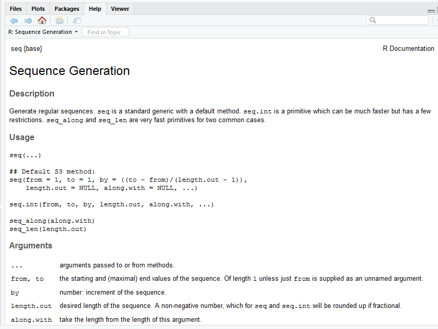

Another function to create a vector with numeric data is the replicate function: rep(x = , times = ), which repeats the argument you provide for ‘x’ as many times as the argument you provide for ‘times’:

rep1 <- rep(1, 4) #This is a command to repeat the value 1 four times
rep1

rep2 <- rep(1:3, 4) #This is a command to repeats the values 1 to 3 four times
rep2

Now, imagine a biomedical experiment with the following setup:

Concentrations of the drug to be tested are: 1 µM, 10 µM, 100 µM and 1000 µM.
For each concentration, measurements are taken at 5 time points: 0, 2, 4, 6, and 8 hours.

9. Write R code to create two vectors below:

A vector named concentrations that repeats each concentration for all time points.
A vector named time_points that sequences the time points for each concentration.

 [1]    1    1    1    1    1   10   10   10   10   10  100  100  100  100  100 1000 1000 1000 1000 1000

 [1] 0 2 4 6 8 0 2 4 6 8 0 2 4 6 8 0 2 4 6 8

4.3 Vectors using rnorm() and runif()

Vectors can be also made with random values using the rnorm() and runif() functions. rnorm() draws numbers from a normal distribution with a mean of 0 and a standard deviation of 1. runif() draws numbers from a uniform distribution in the interval (0, 1).

x <- rnorm(3) # This is a command to return 3 values from a normal distribution
x

y <- rnorm(8) 
y

z <- runif(5) # Uniform random values in the interval (0, 1)
z

4.4 Character vectors

You can also make a vector with character data as follows:

Countries <- c("The Netherlands", "Belgium", "France", "Germany")
Countries

If you want to determine the number of elements that are present in a vector/object, you can use the length(x = ) function, in which you use the vector name as the single argument.

10. Which command returns the number of values in the ‘Countries’ vector?

5. Matrices

A matrix is like a vector because it is also a collection of data elements, but is displayed in rows and columns and is therefore called two-dimensional. As with a vector, a matrix can only contain one type of data (logical, numeric or character).

5.1 Creating matrices

A matrix can be made using the matrix() function, a vector with values, and at least one matrix-dimension. In the next example a matrix will be formed from

The values 1 to 6;
‘nr’ indicates the number of rows that we want, in this case 2;
‘nc’ indicates the number of columns that we want, in this case 3.

matrix1 <- matrix(1:6, nr = 2, nc = 3) #A matrix with values 1 to 6 distributed over 2 rows and 3 columns
matrix1

matrix2 <- matrix(1:6, nr = 3, nc = 2) #A matrix with values 1 to 6 now distributed over 3 rows and 2 columns
matrix2

You can also create separate vectors and combine the vectors to a matrix using the functions rbind() or cbind(). cbind is short for columnbind in which the vectors you provided are put into the columns of a matrix. rbind is short for rowbind and puts the vectors you provide together in the rows of a matrix. Try out this example:

a <- c(1, 2, 3) #vector 1
a

b <- c(4, 5, 6) #vector 2
b

c <- c(7, 8, 9) #vector 3
c

B <- rbind(a, b, c) #combining vector 1, 2 and 3 into rows of a new matrix called B. Note that the capital letter 'B' differs from the lower case 'b'. 
B

C <- cbind(a, b, c) #combining vector 1, 2 and 3 into columns of a new matrix called C.
C

cbind(1:2, 1:2) #columns 1 to 2 of values 1 to 2

rbind(1:2, 1:2) #rows 1 to 2 of values 1 to 2

11. Create the following matrix using cbind(). Next, create the same matrix with rbind():

     [,1] [,2]
[1,]    2    7
[2,]    3   11
[3,]    5   13

You can also use cbind() and rbind() to add rows and columns to an existing matrix.

cbind(B, 7:9) # We now add one extra column with the values 7 to 9

6. Lists

You can use lists to store different data types in one data structure. Lists can contain vectors and matrices but also information such as dates. When you store information in a vector and call the whole vector, R will return everything in that vector in the order you gave it. When you store information in a list and call the whole list, R will return each element separately.

6.1 Creating lists

a <- c("hello", "how", "are", "you", "?") # creates a vector of string values
a # information in the vector is returned in the order you gave it

Create a list using the list() function:

list1 <- list("hello", "how", "are", "you", "?") # creates a list of string values
list1 # each element of the list is returned separately

list2 <- list(name = "Jan", age = 30, is_student = FALSE) # creates a list of character values, numeric values and logical values
list2  # each element of the list is returned separately

12. Create a list named list3 which includes information about “Mieke”, who has won silver on the Olympics 6 times, but never gold (FALSE)

7. Data frames

A data frame is like a matrix because it also contains rows and columns. A data frame is also like lists because it can store different types of data at once. A data frame is a mix between the two. In a data frame, rows correspond with observations (people for example; each row then concerns a different person) and columns correspond with variables (such as age, name and whether the person is in a relationship or not). Each row can contain different types of data but the data in the columns is of the same type (age = numeric, name = character, relationship status = logical). To make a data frame we use the data.frame() function. Before we make a data frame, we need to make different vectors for each column in our data frame.

7.1 Creating data frames

name <- c("Tom", "Nadia", "Anna", "Inge") 
age <- c(24, 20, 21, 23)
relationship <- c(TRUE, FALSE, TRUE, TRUE) # in a data set the question yes or no is marked as TRUE or FALSE
people <- data.frame(name, age, relationship) # placing our vectors into a data frame 
people

Note that the columns have the names of the vectors (name, age, relationship). We can change these with the colnames() function. For example, if we want the column names to have capital letters, we can change this with the following command. Note that the order in which you change the names matters.

colnames(people) <- c("Name", "Age", "Relationship")
people

Within RStudio you can view your data frame by clicking on the data frame in the upper right panel (Environment). The data frame will then be displayed in the upper left panel. You can also use a command to view the data frame:

View(people) #note that the V is a capital letter

8 Factors

A factor is another way to store data. A factor is a data structure that stores so-called categorical data. A categorical variable can belong to a limited number of categories, and thus belongs to a particular finite group. Examples of categorical variables are countries, gender, and occupation. Factors can be ordered or unordered and are an important class for statistical analysis and for plotting. Once created, factors can only contain a pre-defined set of values (categories), known as levels. By default, R sorts levels in alphabetical order. Using the example of a survey in which respondents are asked about their blood type, we will illustrate how factors can be used. Within the categorical variable blood type, there are four different blood types: A, AB, B and O. These blood types are called levels. So, we now have four levels (A = 1, AB = 2, B = 3 and O = 4). We can use these when we survey people for their blood types. In this example we surveyed 8 people in which two had blood type A, three had AB, two had B and one had O.

8.1 Creating factors

We first create a vector containing the answers of the respondents:

bloodtype <- c("A", "AB", "A", "B", "AB", "B", "O", "AB") 
bloodtype

By adding the “quotes”, we make bloodtype a vector with characters. You can confirm that by calling class(Bloodtype).

class(bloodtype)

We now need to transform this character type data to a factor:

bloodtype_factor <- factor(bloodtype)
bloodtype_factor

Here we can see that R returns the levels in alphabetical order.

When comparing other values in the survey between people with different blood types, the factor variable makes it easy to split (stratify) the respondents based on their blood type. You could for example compare the mean age of people with bloodtype “A” with the mean age of all respondents. In addition, factorized data are useful to plot the frequency of different blood types: compare the two commands below.

plot(bloodtype) # returns an error
plot(bloodtype_factor) # plots the blood type distribution

In COO 3, you will learn more about plotting.

13. Create a factor variable named sex. This variable consists of four males and four females, respectively.
Hint, use the rep() function.
14. Combine the factors bloodtype and sex in one data frame.

Summary

In this COO, you have learned to work in RStudio, to perform simple calculations and you have been introduced to the most important data types of R. The questions below might help you to keep the overview for the next COOs:

How do you assign an object?
What are logical, numeric, character and integer data types?
Which command can you use to check the data type of an object?
What are vectors, matrices, lists, data frames and factors? And what types of data can you store in them?
How do you create a vector? How do you create a regular sequence? How do you create a sequence of repeats?
How do you create a matrix?
How do you create a list?
How do you create a data frame? How do you change the column names of a data frame?
How do you create a factor?

Additional exercises

A1. Recreate this next vector and store it in the object species

[1] "human"       "fruit fly"   "rat"         "thale cress"

A2. What type is the object species? What function can you use to determine the type of an object? Use this function to check your answer.

A3. Can you recreate this next vector using vector functions and operations, and store it in the object numbers?

[1] 499 599 699 799

A4. Can you recreate this next data.frame? What are the data types of each column? Can you make sure the kingdom column is a factor?

      species numbers  kingdom
1       human     499 Animalia
2   fruit fly     599 Animalia
3         rat     699 Animalia
4 thale cress     799  Plantae

A5. Rename the three columns to respectively type, count, category.

         type count category
1       human   499 Animalia
2   fruit fly   599 Animalia
3         rat   699 Animalia
4 thale cress   799  Plantae

COO1 - Introduction R - basics

Hugo Kuijf

2024-09-30