In the second computer module, you will learn how to import files into R. In addition, you will learn how to select and order data within objects.

1. Importing data into R studio

We can import files with data into RStudio and start working with them. Common file types are text files, csv (comma-separated values) files, tab delimited files or SPSS files. The first row of these file types generally correspond to the columns of the data frame in R. Data files can be imported through the RStudio interface, as explained in the lecture. However, it is more recommended to import a file through a line of code in your script. For this purpose, you need to specify the file path that indicates the folder in which the file is located on your computer. You can do this by explicitly specifying the full file path each time you use a function to import a file, but also by setting the ‘working directory’ (e.g. the folder on your computer in which the file is stored) at the very top of your script. If you set the working directory, you specify to R in which folder it has to look for (and save) files by default. This helps you to organize your project by working from one folder on your computer in which the original data files are stored and the output generated in your project can be saved (this will be explained later in this course).

1.1 Setting working directory

Create a folder on your computer called Intro_R_COO2 and save the required data files in it. There are a couple of options how you can select your working directory. A possible way is to do this via the R console.

Option 1:

Go to: Session → Set Working Directory → Choose Directory…

R will show a line like this in your Console, which you can copy into your script.

Option 2:

You can tell R where to look using this line of code:

setwd("C:/Users/YourName/Documents/MyProjectFolder")

This path needs to lead to the folder that you have made.

To check in what directory you are currently working, you can use the code:

getwd()

The following data files will be used, so download them:

Save the files in the folder you just created. You can do this by right-clicking on the link and pick ‘Save link as …’ to directly save the file. Note: opening the file and then saving it (e.g. using Excel) may alter the contents! The R scripts that you have created can be saved in this folder as well. Use a proper name for your scripts to prevent chaos. Use for example the date (yy-mm-dd) + file name + version (e.g. 250907_RscriptCOO2_version1).

1.2 Reading a table file with read.table()

The general R function to import data files is the read.table() function, which reads a file and imports it as a data frame. For certain file types, variations of this function are also available—for example, the read.csv() function is designed to import CSV files.

A CSV file contains values separated by commas. If you open the original .txt file, you can see that each line corresponds to a row of data, with each value separated by a comma. By default, read.csv() uses the first line in the file as column names for the data frame in RStudio.

You can import data manually through the RStudio interface by selecting File > Import Dataset > From Text (base) > Import, as shown in the lecture. However, it is recommended to import data by writing the code directly in your script. This way, you can easily find and rerun the command whenever needed. This way, you can easily rerun the import process and maintain a reproducible workflow.

1. Import the Mammogram dataset manually.

When you import the dataset manually, look at the Console panel. You will see the command that RStudio used to import the data. This command uses the read.csv() function. The only argument in this function is the path to your text file, including the file name and extension (e.g., .txt). R automatically assigns the data to an object named after the file, for example:

Mammogram <- read.csv("Mammogram.txt")

Now, let’s import another dataset using the more general function read.table() in your script. The advantage of scripting your import instead of using the manual import is that you can easily find and rerun the command whenever needed. This way, the data will be loaded automatically every time you run your script.

2. Import the Heart_disease data by copying and editing the commands from your Console. Change the object name, the name of the .txt file and change the function to read.table().

When you view your new data (either by clicking on the object in the Environment panel or using the View() function), it is loaded as a data frame with one column and multiple values separated by commas in one cell. read.table() by default uses spaces in the text file to separate columns. Since our data is separated by commas instead of spaces, the data file is not imported properly. In addition, the first row of the file is not used for the column names. Therefore we need to define some new arguments (as shown in the lecture).

3. Adapt the following commands to correctly load the Heart_disease data:

Heart_disease <- read.table("Heart_disease.txt",
                            header = TRUE,
                            sep = ",")
View(Heart_disease)

You can also view the dataset by clicking on the Heart_disease object in the Environment panel (under the Working and History tab).

4. What R data type is used to store text?

In R, text data is typically stored as character type. However, in older versions of R (before version 4.0.0), the read.table() function automatically converts character strings into factors by default.

5. What is the difference between the data types ‘character’ and ‘factor’?

6. Suppose a column in our data frame contains seven patients and the data type is factor. How many levels will this column have?

7. What will happen if we want to add another patient to this column?

We will name our data frame df.patients — the prefix df reminds us this object is a data frame.

8. Import the dataset with the following commands:

df.patients <- read.table("patients.txt",
                          header = TRUE,
                          sep = ",")
df.patients

1.3 Reading a Tab-Delimited File

Take a look at the file “patients_TD.txt”. You’ll notice that, unlike the previous patients file, this one uses tabs instead of commas to separate the data values.

We can still use the read.table() function to import this file, but we need to change the argument sep to "\t", which tells R that the data is tab-delimited.

patients_td <- read.table("patients_TD.txt",
                          header = TRUE,
                          sep = "\t")
head(patients_td)

This will import the data frame just like before.

Alternatively, R has a special function designed for tab-delimited files called read.delim(). It automatically assumes the file uses tabs and that the first line contains column names. So, you can use this simpler command:

patients_td2 <- read.delim("patients_TD.txt")
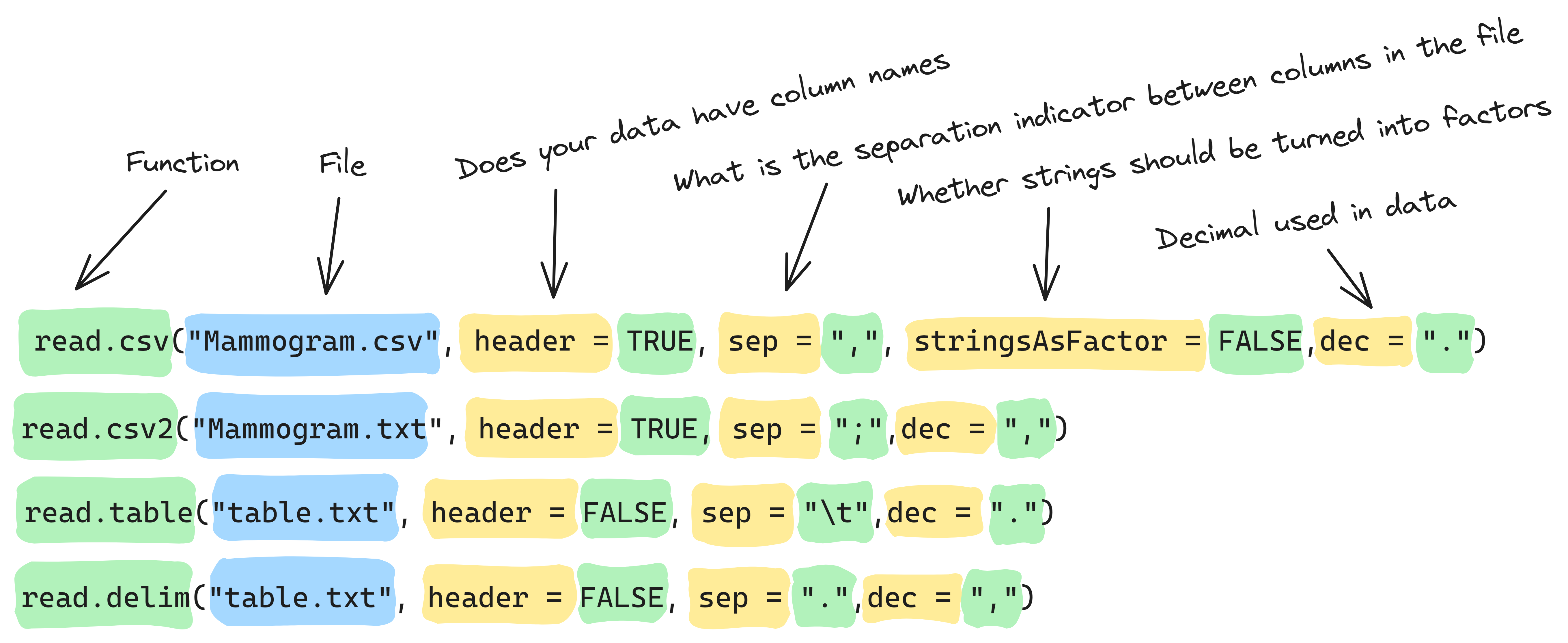
patients_td2

These two functions will give you the same result. Just know that all these read.table type functions assume different default parameters, but you can always specify exactly what you need.

Info graphic about reading files:

1.4 Exploring Your Data

There are different ways to get information on our data. With these functions we can do some quality control, which is very important.

We can view the data frame in our Console by running the following command in our script:

df.patients

This works well for small datasets. For larger datasets, it’s easier to look at just a portion of the data using:

head(df.patients)  # shows the first six rows

To check the type of your data object, use:

class(df.patients)

With the function dim() we can see how many rows and columns there are in this data frame. Or we can see them separately using the nrow() and ncol() functions. The dim() function is different from the length() function used in the previous course (COO1) to determine the number of elements that are present in a vector/object. The length() function is typically applied to a one-dimensional vector and returns the number of elements. The dim() function, on the other hand, is applied to objects with multiple dimensions and gives you the number of rows and columns instead of the number of elements.

dim(df.patients)  # the first being the number of rows, the second being the number of columns
nrow(df.patients)  
ncol(df.patients)

To find out the names of the variables (columns) in your dataset, use:

names(df.patients)

If you want to see a specific number of rows, you can specify that with head() and tail():

head(df.patients, 3)  # first 3 rows
tail(df.patients, 2)  # last 2 rows

A great way to quickly understand the structure of your data frame is:

str(df.patients)

This shows you each variable’s type and a preview of the data.

The summary() function is a powerful tool in R for quickly getting an overview of the key characteristics of your data. When applied to an object, such as a data frame or a numerical vector, the summary() function provides a summary of the data’s central tendency (i.e., mean, median), distribution (i.e., interquartile range, range) and extreme values (i.e., min, max). For example, if you have a data frame named Heart_disease, you can use the summary() function to generate a summary of its variables:

summary(Heart_disease)

The summary() function provides output such as mean, median, minimum, maximum and quartiles for numerical variables, as well as counts and levels for factor variables. This function is particularly useful for an initial exploration of your data and can help you quickly identify potential issues, missing values (NA), outliers, or trends.

2 Selecting data

To select data from any data type, use the index operator []. In one-dimensional data, such as a vector, you provide one index. So, to select the third value of a vector, you use vector[3]. For two-dimensional data, if you want to select one value you need to indicate both the row, and the column. Therefore, you need two indices. data frame[2, 5] selects the value from the second row, fifth column.

2.1 Selecting a subset of a vector

Use the following commands to create a vector and select some values from this vector:

a <- c(2, 3, 4, 5)
a

Select the third element of vector a:

a[3]  # The third element of vector a.

Select the first and third elements:

a[c(1, 3)]  # Returning the first and third elements of vector a.

You can also do calculations with selected elements in a vector:

a[1 + 3]     # Returning the fourth element of a vector. 
a[1] + a[3]  # Adding the first to the third element, returning the sum.

9. Now, select the first two elements of vector a.

You can also select multiple values in a row:

b <- 10:1
b[2:4]  # Returning the second to fourth element of vector b

You can also select a subset of a vector using logical values.

b[b > 3]  # Returning values in the vector of b that are greater than 3

Note that the output is different if you don’t use the index operator [ ] properly.

b > 3  # Which values in the vector of b are greater than 3?

Instead of selecting a subset, you now ask R which values in the vector of b are greater than 3. 10:4 are all greater than 3 and therefore return TRUE, 1, 2 and 3 are smaller or equal to 3 and therefore return FALSE.

Lastly, you can select by excluding values from your vector by using a minus: [-1] selects every value except the first one.

b[-1]  # Returning all values except the first one

10. Select every value of b except the second and sixth.

We can assign new values to a specific subset that we selected. For example we can select the fifth element of vector b and replace it with 0, using the assignment operator <-.

b[5] <- 0

We can also replace larger parts.

b[6:10] <- 9

2.2 Selecting a subset of a matrix

As explained before, to select from a matrix with two dimensions you need to use two indices. You can also select a whole column or row. In that case, we have to specify whether we want to select either the rows or columns by carefully placing commas. The first index is for rows, the second for columns [rows, columns].

First, we make a new matrix with the following vectors:

vector.a <- c(1, 2, 3)  # vector 1
vector.b <- c(4, 5, 6)  # vector 2
vector.c <- c(7, 8, 9)  # vector 3

11. Combine these vectors as columns of a new matrix, called matrix.a.

Now, you can select the first row:

matrix.a[1,] # select row 1 from matrix a

This shows us the first row of the matrix. We can also see both the first and second row by using c(1,2).

matrix.a[c(1,2),]  # select rows 1 and 2 from matrix a

Put your indices after the comma to select columns:

matrix.a[,c(1,3)]  # select columns 1 and 3 from matrix a

12. Now, select the value in the third row, second column of matrix.a.

13. Next, select the value in the second row, first column of matrix.a.

14. Can you describe what this next line of code does to matrix.a?

matrix.a[2,1] <- 999

2.3 Selecting a subset of a data frame

When working with data frames in R, there are different ways to select parts of your data. Knowing how to select rows, columns, or specific cells is essential for data analysis.

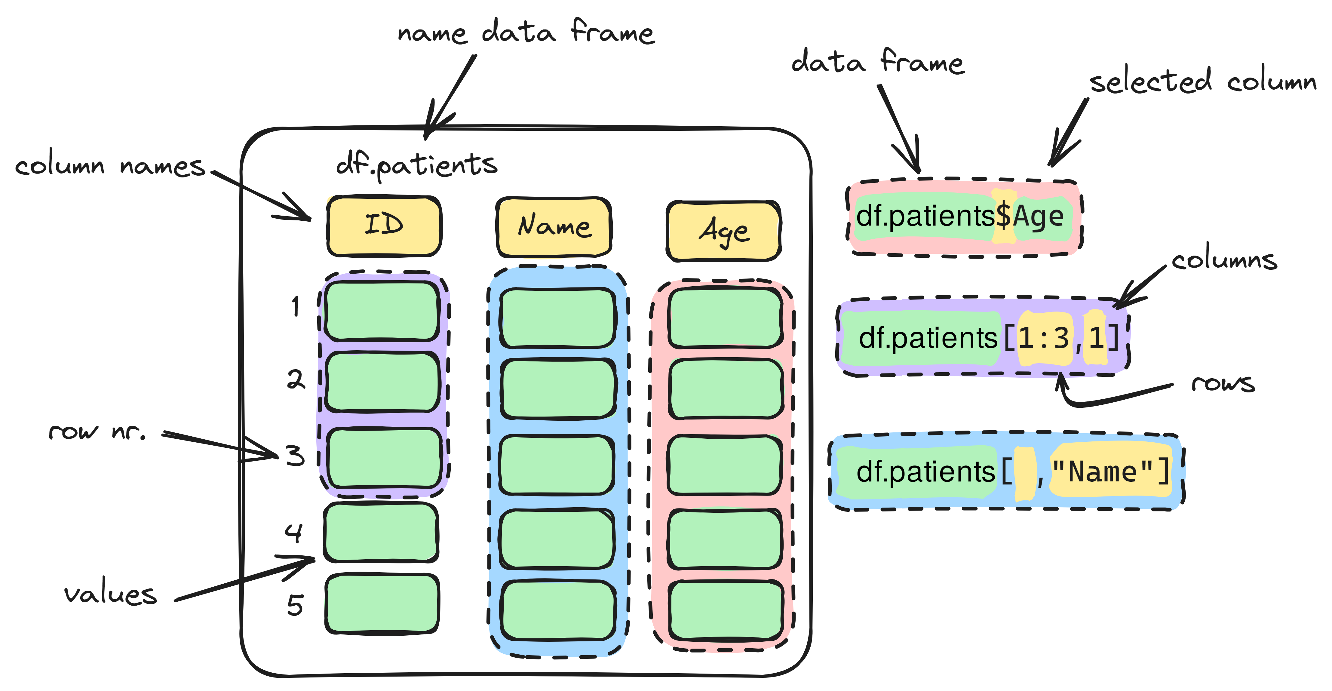
There are multiple ways to select data from a data frame in R. You can use:

The index operator []
The dollar sign $
The collumn name as a character string inside []

df.patients[2,]  # selecting row 2
df.patients[,4]  # selecting column 4
df.patients[,"Diagnosis"]  # selecting the information in the column called Diagnosis
df.patients$Diagnosis  # selecting the information in the column called Diagnosis

15. Use the class() function to check the type of data returned by each of these commands.

class(df.patients[2, ])   # What class is returned by selecting row 2?

You can use selection commands with summary functions like mean(), min(), and max() to calculate statistics for your data.

16. Calculate the mean age in the df.patients data frame using the summary() function.

17. Calculate the minimum and maximum age in the Heart_disease data frame, using the dollar sign “$” to get suggestions for the column names.

We can also select data using logical operators, explained in the previous COO. The expressions created with logical operators are also called Boolean expressions.

Example: To find patients older than 40:

above40 <- df.patients$Age > 40

This creates Boolean expression, (TRUE or FALSE; 1 or 0) values indicating whether each patient meets the condition.

Use this logical vector to select only those patients:

df.patients[above40, "Patient_ID"]  # for each row of the data frame the boolean 'above40' is checked (TRUE or FALSE) and the Paient_ID is displayed (TRUE) or not (FALSE)

This returns the patient ID’s of people above the age of 40.

18. Produce the diagnosis of patients who are under 45 in a similar way.

Info graphic about selecting:

3. Sorting and ordering data

Next, we will learn about the sort() and order() functions in R.

The sort() function takes a vector of values and returns those values arranged from smallest to largest, or in alphabetical order if the values are characters.
The order() function, on the other hand, returns the positions (indices) that would sort the data. In other words, it tells you the order in which to arrange the original data to get a sorted result.

For example, consider the vector:

# Define a character vector
alphabet <- c("c", "a", "b")

# sort() returns the sorted values
sort(alphabet)
# [1] "a" "b" "c"

# order() returns the indices that would sort the vector
order(alphabet)
# [1] 2 3 1
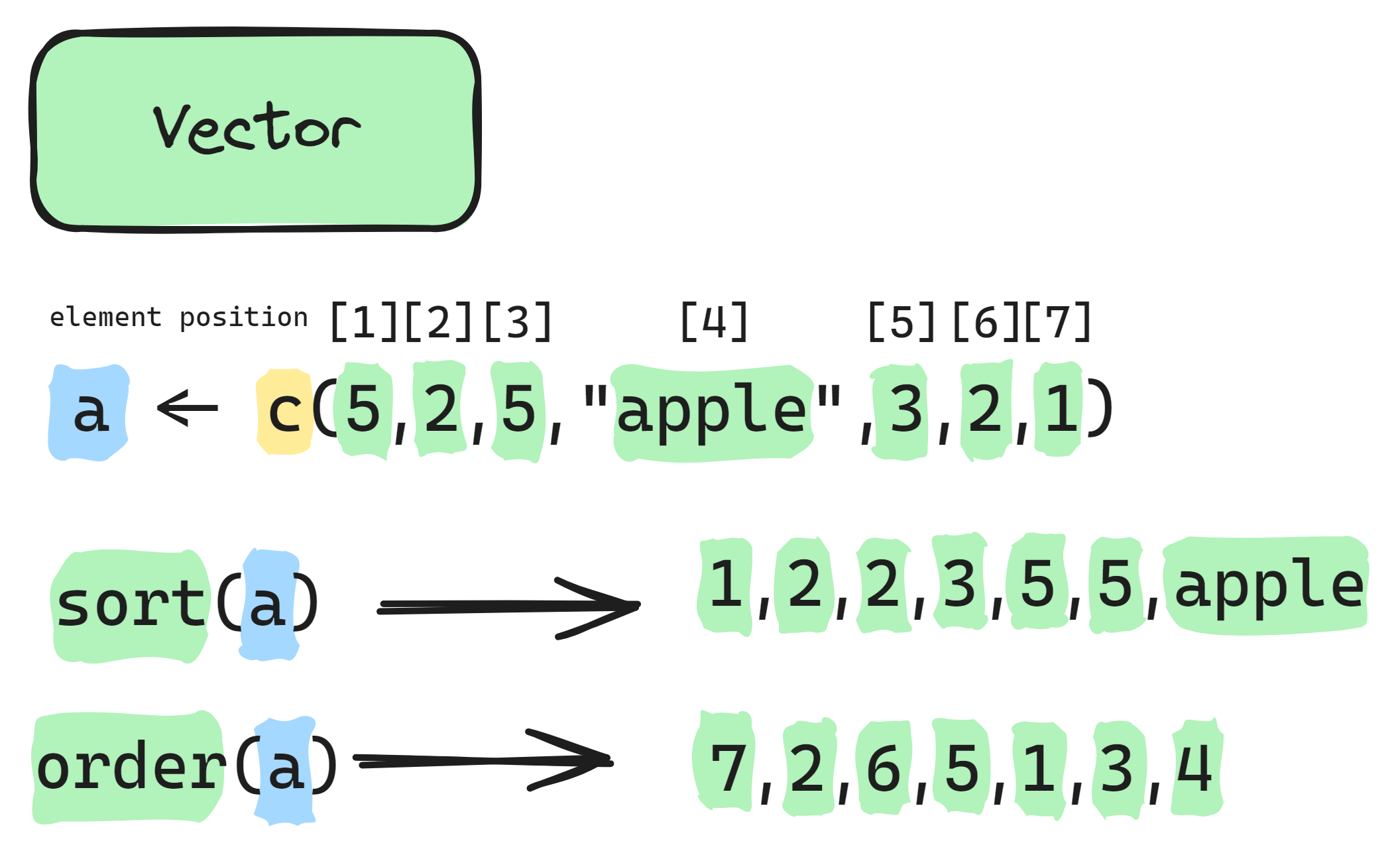
# Because the second value ("a") is the lowest in the alphabet, then the third value ("b"), and then the first value ("c").

sort() gives the values from lowest to highest (or alphabetically), order() gives the positions of these sorted values in the original vector.

Info graphic about sorting and ordering vector:

An example of data sorting:

sort(Heart_disease$age)                     # From low to high
sort(Heart_disease$age, decreasing = TRUE)  # From high to low

Note: Using sort() only returns the sorted vector; it does not change the order of rows in the original data frame.

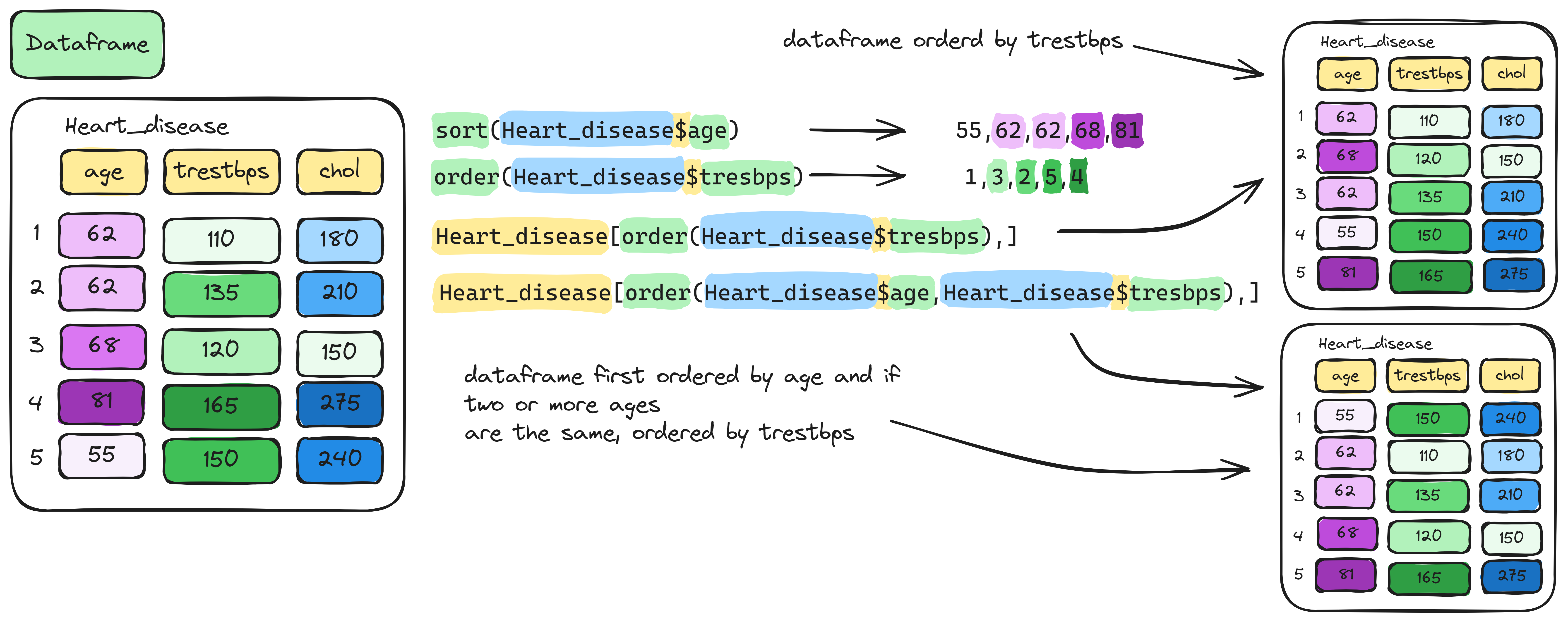
To rearrange the whole data frame according to the sorted order of a column, use the order() function inside row indexing:

age_ordered <- order(Heart_disease$age) 
age_sorted <- Heart_disease[age_ordered,]

Here, order(Heart_disease$age) returns the row indices that would sorts the ages numerically. We use this to reorder the entire data frame by age.

19. Create a new data frame called Cholesterol_sorted, sorted by the amount of cholesterol with the Heart_disease data frame:

The following commands were used in the lecture for the iris data set, use it now for the Heart_disease data set:

volgorde <- order(iris_dataset$sepal_width)
iris_sorted <- iris_dataset[volgorde,]
iris_sorted <- iris_dataset[order(iris_dataset$sepal_width),]
iris_sorted <- iris_dataset[order(iris_dataset$flower, iris_dataset$sepal_width),]

iris_sorted <- iris_dataset[order(iris_dataset$flower, iris_dataset$sepal_width,
                                  decreasing = c(FALSE, TRUE), method = "radix"),]

The iris_sorted data frame has the iris_dataset data first sorted in increasing order on flower name, and then in decreasing order on sepal width.

20. Create a new data frame in which you sort the Heart_disease data first in decreasing order on sex, and then in increasing order on age.

Info graphic about sorting and ordering data frame:

4. Missing values

Sometimes when you import a data set or manipulate one it can have missing information. Missing data is displayed with a NA value (not available). Some calculation performed on a column with missing like with the mean() function it could give you back NA as response instead of the calculated mean. Conclusions drawn with a data frame containing NA’s could be misleading. Always view the data frame you import to check if it was done right. NA’s can also be removed what is done frequently .

Let’s work with the incomplete Heart_disease data set. Lets import the data set and save if under a new name.

# Summary of all columns (will show NA if present)
summary(Heart_disease_incomplete)

# Find the row(s) where restecg is NA
which(is.na(Heart_disease_incomplete$restecg))

# Remove rows that contain NA (creates a new clean data frame)
heart_clean <- na.exclude(Heart_disease_incomplete)

# Calculate mean of restecg (returns NA)
mean(Heart_disease_incomplete$restecg)

# Calculate mean, ignoring NA values
mean(Heart_disease_incomplete$restecg, na.rm = TRUE)

Note that the na.exclude() function itself does not remove the row containing NA, only if you assign it to a new object. This new object will contain the original data set minus the row containing NA, so will have one observation (row) less than the original data set. You can also check the number of NA values with the sum(is.na()) function.

21. Check the number of NA values in the Heart_disease, Heart_disease_incomplete and heart_clean data frames.

22. Explain the difference between using the function na.exclude() or the argument na.rm = TRUE.

5. Saving Output and R Script

Saving your work in R is essential for reproducibility, future use, or sharing with others. This includes saving both your data/output and your R scripts.

To save your data and output in the desired folder, it is important to set the working directory, as previously discussed. You can additionally check this with the getwd() function. If the working directory is not set, you need to provide the entire path to the folder in which you aim to save the files.

It is essential to manage your working directory properly to ensure that R can access the files it needs.

5.1 Write data frame to a file

The write.table() or write.csv() functions are used to save data frames or matrices as text files. This is helpful for sharing data with others or importing it to other software programmes. For example:

mydata <- data.frame(Name = c("Alice", "Bob", "Charlie"),
                     Age = c(25, 30, 28))
write.csv(mydata, file = "mydata.csv", row.names = FALSE)

This saves the mydata data frame as a CSV file named mydata.csv. You can import your .csv file for example in Excel via ‘import data’.

5.2 Saving R script

R scripts - in which you write your code in the RStudio’s script editor - can be saved with an .R extension. Saving your R script is important for reproducibility and sharing with others. In the top of your window click the ‘disk icon’ to save your R script. Or click File → Save As, shortcut is ctrl + s.

Your script will be saved with a .R extension by default (e.g., OZM_COO2_V1.R), which you can reopen later to rerun your analysis.

6 Extra assignment

Import the BloodResults.txt file as a data frame and check whether it worked correctly.
How many rows and columns does the data frame have?
What are the column names?
What does the first part of this data frame look like?
Provide a summary of the data.
Are there biologically implausible values (e.g., negative or extreme CRP above 300 or HbA1 above 20)?
How many NA values are present in the dataset?
What are the mean CRP and HbA1c levels (excluding NA values)?
Create a new data frame that excludes rows containing NA values.
Create logical vectors identifying patients with CRP > 100 or HbA1c > 14.
Which values exceed these thresholds?
Values < 0 are not sensible. Create logical vectors for CRP and HbA1c for these values.
The -4.0 in the data set is a typo. The measurement was checked in the patient dossier and should be 4.0 instead of -4.0. Change the typo to the correct value in R. Try to use the which function to find the position of the typo. Hint: use arr.ind = TRUE.
Create a vector of CRP values sorted from lowest to highest.
Create a vector of HbA1c values sorted from highest to lowest.
Create a new data frame sorted first by CRP (ascending), then by HbA1c (ascending).
Recalculate the average CRP and HbA1c levels in the corrected data.
What is the highest CRP value in the dataset?
Which row(s) contain this highest value?
What is the name of the patient with the highest CRP level?
What is the name of the patient with the lowest HbA1c level?

COO2 - Introduction R - importing, selecting, ordering, and missing data

2025-09-02